Automated Load and Export Pipelines in Autonomous Database

Introduction
Data Lakehouse combines the agility and low costs of Data Lake, with the data integrity and analytics power of Data Warehouse. In Oracle Cloud, the data lake part of the Lakehouse is usually implemented in the OCI Object Storage, while the data warehouse is provided by the Autonomous Data Warehouse.
With Autonomous Data Warehouse, you can easily map structured and semi-structured data in OCI Object Storage to relational tables using external tables and DBMS_CLOUD package. This approach allows you to keep data in the OCI Object Storage and use Autonomous Data Warehouse as query and analytical engine.
However, if you need to deliver low latency queries to many concurrent users, accessing data in the OCI Object Storage might not give you the required performance. In this case, you may decide to load data into the Autonomous Data Warehouse and use the power of ADW, such as Exadata Storage, indexing, or columnar compression, for better performance.
Recently, Oracle introduced a new feature called Data Pipelines (see Using Oracle Data Pipelines for Continuous Data Import and Export in Autonomous Database from Nilay Panchal), which supports automated, simple loading of data from the OCI Object Storage and other supported object stores into Autonomous Database. Data Pipelines regularly check for new objects in the object storage and they load these objects into designated tables.
And, even better, Data Pipelines support also automated, incremental export of data from Autonomous Database into an object storage. So you can use this feature not only for simple loading of data from a Data Lake into the Autonomous Data Warehouse, but also for publishing data from Autonomous Data Warehouse into an object storage based Data Lake.
If you do not need to apply transformations, and if the time based scheduling of import and export pipelines is acceptable, Data Pipelines is the simplest method for automated loading of data from an object storage to Autonomous Database, and for publishing information from the Autonomous Database to an object storage.
Use Case
Overview
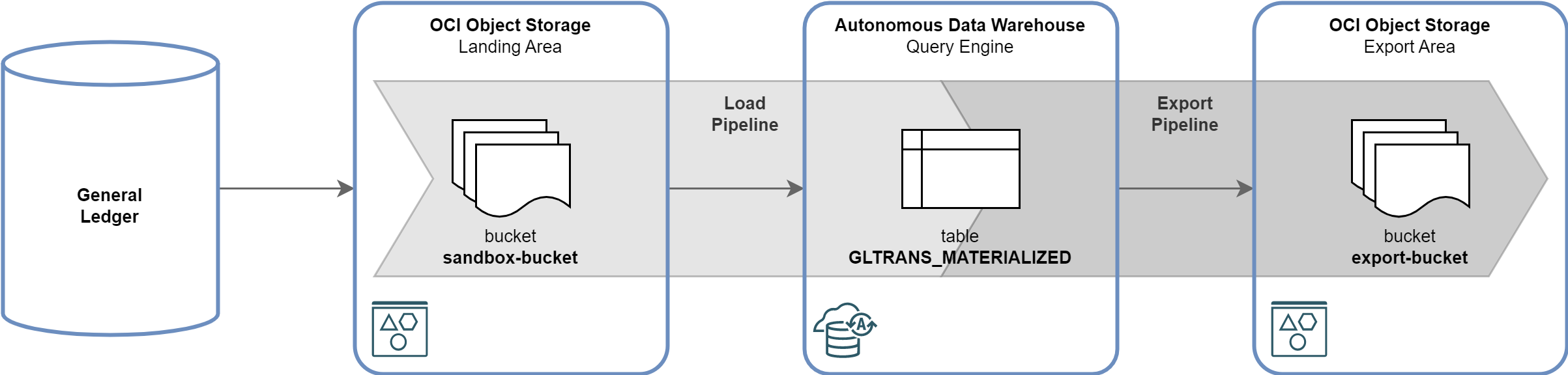
In this post I will demonstrate how to create and monitor a load pipeline to import General Ledger data from OCI Object Storage into Autonomous Data Warehouse. I will also show how subset of this data can be regularly exported back from the Autonomous Data Warehouse to OCI Object Storage. The scenario is depicted below:
-
GL Journal Entries are extracted every 30 minutes from the General Ledger, formatted into Parquet files, and saved as objects in the OCI Object Storage, in the
sandbox-bucket. The extraction process is out of scope of this post. -
GL Journal Entries are automatically loaded via Load Pipeline from OCI Object Storage into the Autonomous Data Warehouse table
GLTRANS_MATERIALIZED. The load happens every 20 minutes. -
GL Journal Entries are incrementally exported from the Autonomous Data Warehouse table
GLTRANS_MATERIALIZEDback to OCI Object Storage bucketexport-bucketvia Export Pipeline. The export process runs every 60 minutes.
Source Data Objects
Object names with GL Journal Entries extracted from the General Ledger look as follows:
[opc@bastionhost scripts]$ oci os object list --bucket-name sandbox-bucket --prefix gl/trans \
--query 'data[].{name:name, size:size, "time-created":"time-created", "time-modified":"time-modified"}' \
--output table --all
+---------------------------------------------------------+---------+----------------------------------+----------------------------------+
| name                                                    | size    | time-created                     | time-modified                    |
+---------------------------------------------------------+---------+----------------------------------+----------------------------------+
| gl/trans/gl_trans_20230323_100005_990544_000000.parquet | 4080742 | 2023-03-23T10:00:10.524000+00:00 | 2023-03-23T10:00:10.524000+00:00 |
| gl/trans/gl_trans_20230323_103005_805517_000000.parquet | 4036019 | 2023-03-23T10:30:10.242000+00:00 | 2023-03-23T10:30:10.242000+00:00 |
| gl/trans/gl_trans_20230323_110006_443909_000000.parquet | 4104642 | 2023-03-23T11:00:11.243000+00:00 | 2023-03-23T11:00:11.243000+00:00 |
| gl/trans/gl_trans_20230323_113006_542490_000000.parquet | 4070642 | 2023-03-23T11:30:11.033000+00:00 | 2023-03-23T11:30:11.033000+00:00 |
| gl/trans/gl_trans_20230323_120006_288388_000000.parquet | 4014379 | 2023-03-23T12:00:10.708000+00:00 | 2023-03-23T12:00:10.708000+00:00 |
| gl/trans/gl_trans_20230323_123006_066852_000000.parquet | 3993469 | 2023-03-23T12:30:10.433000+00:00 | 2023-03-23T12:30:10.433000+00:00 |
...
+---------------------------------------------------------+---------+----------------------------------+----------------------------------+
prefixes: []
[opc@bastionhost scripts]$
Source Data Structure
Objects with GL Journal Entries are in the Parquet format. Structure of the objects, as
reported by Python’s pandas, is the following:
>>> import pandas
>>> df = pandas.read_parquet('gl_trans_20230323_100005_990544_000000.parquet')
>>> df.info()
<class 'pandas.core.frame.DataFrame'>
RangeIndex: 51275 entries, 0 to 51274
Data columns (total 25 columns):
 #   Column                               Non-Null Count  Dtype
---  ------                               --------------  -----
 0   journal_header_source_code           51275 non-null  object
 1   journal_external_reference           51275 non-null  object
 2   journal_header_description           51275 non-null  object
 3   period_code                          51275 non-null  object
 4   period_date                          51275 non-null  datetime64[ns]
 5   currency_code                        51275 non-null  object
 6   journal_category_code                51275 non-null  object
 7   journal_posted_date                  51275 non-null  datetime64[ns]
 8   journal_created_date                 51275 non-null  datetime64[ns]
 9   journal_created_timestamp            51275 non-null  datetime64[ns]
 10  journal_actual_flag                  51275 non-null  object
 11  journal_status                       51275 non-null  object
 12  journal_header_name                  51275 non-null  object
 13  reversal_flag                        51275 non-null  object
 14  reversal_journal_header_source_code  51275 non-null  object
 15  journal_line_number                  51275 non-null  int64
 16  account_code                         51275 non-null  object
 17  organization_code                    51275 non-null  object
 18  project_code                         51275 non-null  object
 19  journal_line_type                    51275 non-null  object
 20  entered_debit_amount                 51275 non-null  float64
 21  entered_credit_amount                51275 non-null  float64
 22  accounted_debit_amount               51275 non-null  float64
 23  accounted_credit_amount              51275 non-null  float64
 24  journal_line_description             51275 non-null  object
dtypes: datetime64[ns](4), float64(4), int64(1), object(16)
memory usage: 9.8+ MB
>>>
Target Data Model
The target table GLTRANS_MATERIALIZED contains all the data fields available in source objects.
create table gltrans_materialized (
  journal_header_source_code                      varchar2(200),
  journal_external_reference                      varchar2(200),
  journal_header_description                      varchar2(200),
  period_code                                     varchar2(200),
  period_date                                     timestamp(6),
  currency_code                                   varchar2(200),
  journal_category_code                           varchar2(200),
  journal_posted_date                             timestamp(6),
  journal_created_date                            timestamp(6),
  journal_created_timestamp                       timestamp(6),
  journal_actual_flag                             varchar2(200),
  journal_status                                  varchar2(200),
  journal_header_name                             varchar2(200),
  reversal_flag                                   varchar2(200),
  reversal_journal_header_source_code             varchar2(200),
  journal_line_number                             number,
  account_code                                    varchar2(200),
  organization_code                               varchar2(200),
  project_code                                    varchar2(200),
  journal_line_type                               varchar2(200),
  entered_debit_amount                            number,
  entered_credit_amount                           number,
  accounted_debit_amount                          number,
  accounted_credit_amount                         number,
  journal_line_description                        varchar2(200)
)
/
Load Pipelines
Prerequisites
Before you can create and run a Data Pipeline, it is necessary to authenticate and authorize the Autonomous Data Warehouse instance to read buckets, and read and write objects. With Resource Principle authentication, the following must be in place:
- OCI Dynamic Group that contains ADW instance.
- OCI Policy, which allows the Dynamic Group to read object-family, manage objects, and inspect compartments.
- Resource Principal Credential
OCI$RESOURCE_PRINCIPALin the ADW database.
Furthermore, the target table must be created in the ADW database.
Create Pipeline
The load pipeline LOAD_GLTRANS is created in two steps. The first step creates and
names the pipeline.
begin
  dbms_cloud_pipeline.create_pipeline(
    pipeline_name => 'LOAD_GLTRANS',
    pipeline_type => 'LOAD',
    description   => 'Load data into GLTRANS_MATERIALIZED table'
  );
end;
/
The second step configures the required attributes, such as credential, location and format
of source objects, name of the target table, and frequency of load (in minutes). The
attributes defining location and format of source objects are the same as the ones used in
DBMS_CLOUD package.
begin
  dbms_cloud_pipeline.set_attribute(
    pipeline_name => 'LOAD_GLTRANS',
    attributes    => json_object(
      'credential_name' value 'OCI$RESOURCE_PRINCIPAL',
      'location' value 'https://objectstorage.uk-london-1.oraclecloud.com/n/<namespace>/b/sandbox-bucket/o/gl/trans',
      'table_name' value 'GLTRANS_MATERIALIZED',
      'format' value '{"type":"parquet"}',
      'priority' value 'high',
      'interval' value '20')
  );
end;
/
Once the pipeline is created, you can verify its attributes in dictionary views
USER_CLOUD_PIPELINES and USER_CLOUD_PIPELINE_ATTRIBUTE.
I did not have to provide the field_list attribute specifying fields in the source
files and their data types. The reason is that the source objects are in Parquet format
and field names and data types are derived from the Parquet structure. For text formats,
such as CSV, the field_list is required.
Test Pipeline
To test the load pipeline, run the pipeline once, explore and validate the results. In other words, check there are no errors and that all data from OCI Object Storage is loaded into the target table.
begin
  dbms_cloud_pipeline.run_pipeline_once(
    pipeline_name => 'LOAD_GLTRANS'
);
end;
/
Once the pipeline is successfuly tested, you can reset the metadata and (optionally) truncate the target table.
begin
  dbms_cloud_pipeline.reset_pipeline(
    pipeline_name => 'LOAD_GLTRANS',
    purge_data => TRUE
);
end;
/
Start Pipeline
To start the pipeline, run the following command. This will execute the pipeline every 20
minutes, as specified by the pipeline attribute interval. The start_date attribute is
optional - when not specified, the pipeline will start immediately.
begin
  dbms_cloud_pipeline.start_pipeline(
    pipeline_name => 'LOAD_GLTRANS',
    start_date => to_timestamp('2023/03/23 11:12','YYYY/MM/DD HH24:MI')
  );
end;
/
Monitor Pipeline
Running pipeline may be monitored by querying dictionary view USER_CLOUD_PIPELINE_HISTORY.
This view contains one line for every successful or failed execution of the pipeline. Note
the 20 minutes interval between successive executions of the pipeline.
SQL> select pipeline_id,
  2    pipeline_name,
  3    status,
  4    error_message,
  5    to_char(start_date, 'YYYY/MM/DD HH24:MI:SS') as start_date,
  6    to_char(end_date, 'YYYY/MM/DD HH24:MI:SS') as end_date,
  7    round(extract(hour from end_date-start_date)*60*60+extract(minute from end_date-start_date)*60+extract(second from end_date-start_date),0) as duration_sec
  8  from user_cloud_pipeline_history
  9  where pipeline_name = 'LOAD_GLTRANS'
 10  order by start_date
 11* /

   PIPELINE_ID PIPELINE_NAME    STATUS       ERROR_MESSAGE    START_DATE             END_DATE                  DURATION_SEC
______________ ________________ ____________ ________________ ______________________ ______________________ _______________
             3 LOAD_GLTRANS     SUCCEEDED                     2023/03/23 11:22:04    2023/03/23 11:22:05                  1
             3 LOAD_GLTRANS     SUCCEEDED                     2023/03/23 11:42:04    2023/03/23 11:42:08                  4
             3 LOAD_GLTRANS     SUCCEEDED                     2023/03/23 12:02:03    2023/03/23 12:02:06                  3
             3 LOAD_GLTRANS     SUCCEEDED                     2023/03/23 12:22:03    2023/03/23 12:22:04                  1
             3 LOAD_GLTRANS     SUCCEEDED                     2023/03/23 12:42:03    2023/03/23 12:42:06                  3
...
If you want to see objects which were imported, you need to query the PIPELINE$X$YSTATUS
table that is created for every pipeline. This table shows when a particular object is
loaded, how big it is, what is the load status, and how many rows were loaded. Note the
name of the status table is available in dictionary view
USER_CLOUD_PIPELINES.STATUS_TABLE.
SQL> select id
  2  , name as object_name
  3  , bytes as object_bytes
  4  , to_char(last_modified, 'YYYY/MM/DD HH24:MI:SS') as object_last_modified
  5  , status
  6  , error_code
  7  , error_message
  8  , to_char(start_time, 'YYYY/MM/DD HH24:MI:SS') as start_time
  9  , to_char(end_time, 'YYYY/MM/DD HH24:MI:SS') as end_time
 10  , round(extract(hour from end_time-start_time)*60*60+extract(minute from end_time-start_time)*60+extract(second from end_time-start_time),0) as duration_sec
 11  , rows_loaded
 12  from PIPELINE$3$76_STATUS
 13  order by start_time
 14* /

   ID OBJECT_NAME                                          OBJECT_BYTES OBJECT_LAST_MODIFIED    STATUS          ERROR_CODE ERROR_MESSAGE    START_TIME             END_TIME                  DURATION_SEC    ROWS_LOADED
_____ _________________________________________________ _______________ _______________________ ____________ _____________ ________________ ______________________ ______________________ _______________ ______________
    1 gl_trans_20230323_100005_990544_000000.parquet            4080742 2023/03/23 10:00:10     COMPLETED                                   2023/03/23 11:12:15    2023/03/23 11:12:19                  3          51275
    2 gl_trans_20230323_103005_805517_000000.parquet            4036019 2023/03/23 10:30:10     COMPLETED                                   2023/03/23 11:12:19    2023/03/23 11:12:21                  2          50588
    3 gl_trans_20230323_110006_443909_000000.parquet            4104642 2023/03/23 11:00:11     COMPLETED                                   2023/03/23 11:12:21    2023/03/23 11:12:23                  3          51533
    4 gl_trans_20230323_113006_542490_000000.parquet            4070642 2023/03/23 11:30:11     COMPLETED                                   2023/03/23 11:42:05    2023/03/23 11:42:07                  2          51123
    5 gl_trans_20230323_120006_288388_000000.parquet            4014379 2023/03/23 12:00:10     COMPLETED                                   2023/03/23 12:02:04    2023/03/23 12:02:06                  2          50279
    6 gl_trans_20230323_123006_066852_000000.parquet            3993469 2023/03/23 12:30:10     COMPLETED                                   2023/03/23 12:42:04    2023/03/23 12:42:06                  2          50013
...
Object names in this table do not contain the prefix specified in the location parameter
of the pipeline.
Monitor Data
You can easily compare data loaded into target table via load pipeline with data in the OCI Object Storage. To do so, you need to define an external table using the same location and format as the pipeline, and then run SQL query to compare the target table with this external table.
For our use case the external table will look like this:
begin
  dbms_cloud.create_external_table(
    table_name => 'GLTRANS_EXTERNAL',
    credential_name => 'OCI$RESOURCE_PRINCIPAL',
    file_uri_list => 'https://objectstorage.uk-london-1.oraclecloud.com/n/<namespace>/b/sandbox-bucket/o/gl/trans/*.parquet',
    format => json_object(
      'type' value 'parquet',
      'schema' value 'first'
    )
  );
end;
/
And the following query will compare number of rows for every load.
SQL> select nvl(e.ext_timestamp, m.mat_timestamp) as created_timestamp,
  2    e.ext_count as external_table_count,
  3    m.mat_count as materialized_table_count,
  4    case when e.ext_count = m.mat_count then 'OK' else 'MISSING' end as status
  5  from (
  6    select to_char(journal_created_timestamp,'YYYY/MM/DD HH24:MI') as ext_timestamp,
  7      count(*) as ext_count
  8    from gltrans_external
  9    group by to_char(journal_created_timestamp,'YYYY/MM/DD HH24:MI')
 10  ) e
 11  full outer join
 12  (
 13    select to_char(journal_created_timestamp,'YYYY/MM/DD HH24:MI') as mat_timestamp,
 14      count(*) as mat_count
 15    from gltrans_materialized
 16    group by to_char(journal_created_timestamp,'YYYY/MM/DD HH24:MI')
 17  ) m
 18  on (e.ext_timestamp = m.mat_timestamp)
 19  order by nvl(e.ext_timestamp, m.mat_timestamp)
 20* /

CREATED_TIMESTAMP       EXTERNAL_TABLE_COUNT    MATERIALIZED_TABLE_COUNT STATUS
____________________ _______________________ ___________________________ _________
2023/03/23 10:00                       51275                       51275 OK
2023/03/23 10:30                       50588                       50588 OK
2023/03/23 11:00                       51533                       51533 OK
2023/03/23 11:30                       51123                       51123 OK
2023/03/23 12:00                       50279                       50279 OK
2023/03/23 12:30                       50013                       50013 OK
...
Import Command
Oracle does not publish how exactly are the object storage objects loaded. But, by looking at the SQL statements running in the ADW database, you can see that load pipeline imports one object at time, using direct path with parallel DML. Example of the insert statement is below.
INSERT /*+ append enable_parallel_dml */ INTO "ADMIN"."GLTRANS_MATERIALIZED"
SELECT * FROM "ADMIN"."PIPELINE$3$JCE5UIMPM8US9C82OS4D"
EXTERNAL MODIFY ( LOCATION ('https://objectstorage.uk-london-1.oraclecloud.com/n/<namespace>/b/sandbox-bucket/o/gl/trans/gl_trans_20230328_063003_560921_000000.parquet') )
Export Pipelines
Create Pipeline
Export pipeline is created the same way as load pipeline, with pipeline_type set to EXPORT.
begin
  dbms_cloud_pipeline.create_pipeline(
    pipeline_name => 'EXPORT_GLTRANS',
    pipeline_type => 'EXPORT',
    description   => 'Export data from GLTRANS_MATERIALIZED table'
  );
end;
/
When configuring the export pipeline, you have to decide if to export the whole table (via
parameter table_name), or if to export data by specifying database query (via parameter
query). Furthermore, you can define parameter key_column, which specifies column in
the table or query that will be used for incremental export. If this parameter is not
specified, every execution of Export Pipeline will export all rows present in the table.
The following configuration will export subset of columns from table
GLTRANS_MATERIALIZED to JSON files every 60 minutes. The export will be incremental,
using column JOURNAL_CREATED_TIMESTAMP.
declare
  query_stmt varchar2(4000) := '
select period_code, period_date, currency_code, journal_category_code, journal_posted_date,
  journal_created_date, journal_created_timestamp, journal_actual_flag, journal_status,
  journal_header_name, reversal_flag, journal_line_number, account_code, organization_code,
  project_code, journal_line_type, entered_debit_amount, entered_credit_amount,
  accounted_debit_amount, accounted_credit_amount
from gltrans_materialized
';
begin
  dbms_cloud_pipeline.set_attribute(
    pipeline_name => 'EXPORT_GLTRANS',
    attributes    => json_object(
      'credential_name' value 'OCI$RESOURCE_PRINCIPAL',
      'location' value 'https://objectstorage.uk-london-1.oraclecloud.com/n/<namespace>/b/export-bucket/o/gl/trans/exp_gltrans',
      'query' value query_stmt,
      'key_column' value 'JOURNAL_CREATED_TIMESTAMP',
      'format' value '{"type":"json"}',
      'priority' value 'high',
      'interval' value '60')
  );
end;
/
Incremental Export
When you define the parameter key_column, export pipeline will extract data
incrementally. In other words, every execution of the pipeline will extract data that was
inserted or updated since the previous execution. The following where condition is used
for the incremental extraction.
WHERE
  SYS_EXTRACT_UTC(CAST(<key_column> AS TIMESTAMP) AT TIME ZONE 'UTC')  > <previous_timestamp> AND
  SYS_EXTRACT_UTC(CAST(<key_column> AS TIMESTAMP) AT TIME ZONE 'UTC')  <= <current_timestamp>
<key_column>is casted as timestamp and converted to UTC time.<current_timestamp>is timestamp of the current SCN (i.e., as of the beginning of the export) in UTC time.<previous_timestamp>is timestamp in UTC time from the previous pipeline execution.
Have this in mind when considering if to export data incrementally and which column to use
as key_column. Also, be aware that data produced by in-flight transactions, not committed
when the export starts, will not be visible to the export and will not be therefore
exported. Ideally, the export should happen at time when there are no active transactions
in table being exported.
Exported Data
The above export pipeline produces objects with names containing the prefix (from the
location attribute), timestamp of the extraction, and suffix denoting the type of
object. For every execution, the export pipeline produces multiple export files, with size
around 10MB.
[opc@bastionhost scripts]$ oci os object list --bucket-name export-bucket --prefix gl/trans \
> --query 'data[].{name:name, size:size, "time-created":"time-created", "time-modified":"time-modified"}' \
> --output table --all
+----------------------------------------------------+----------+----------------------------------+----------------------------------+
| name                                               | size     | time-created                     | time-modified                    |
+----------------------------------------------------+----------+----------------------------------+----------------------------------+
| gl/trans/exp_gltrans_1_20230327T171010563626Z.json | 10485171 | 2023-03-27T17:10:17.218000+00:00 | 2023-03-27T17:10:17.218000+00:00 |
| gl/trans/exp_gltrans_1_20230327T171017303386Z.json | 10485567 | 2023-03-27T17:10:18.018000+00:00 | 2023-03-27T17:10:18.018000+00:00 |
| gl/trans/exp_gltrans_1_20230327T171018102865Z.json | 10485381 | 2023-03-27T17:10:18.516000+00:00 | 2023-03-27T17:10:18.516000+00:00 |
| gl/trans/exp_gltrans_1_20230327T171018609955Z.json | 10485631 | 2023-03-27T17:10:21.868000+00:00 | 2023-03-27T17:10:21.868000+00:00 |
| gl/trans/exp_gltrans_1_20230327T171021952794Z.json | 10485220 | 2023-03-27T17:10:22.227000+00:00 | 2023-03-27T17:10:22.227000+00:00 |
| gl/trans/exp_gltrans_1_20230327T171022312045Z.json | 10485199 | 2023-03-27T17:10:22.619000+00:00 | 2023-03-27T17:10:22.619000+00:00 |
...
+----------------------------------------------------+----------+----------------------------------+----------------------------------+
prefixes: []
The export pipeline with JSON format produces files as JSON Lines; with one database record corresponding to 1 JSON document as shown below. The example below is formatted for better readibility; in reality, every JSON document is stored on a single line.
{
  "PERIOD_CODE": "202303",
  "PERIOD_DATE": "2023-03-31T10:00:05.990544",
  "CURRENCY_CODE": "USD",
  "JOURNAL_CATEGORY_CODE": "RXC",
  "JOURNAL_POSTED_DATE": "2023-03-23T10:00:05.990544",
  "JOURNAL_CREATED_DATE": "2023-03-23T10:00:05.990544",
  "JOURNAL_CREATED_TIMESTAMP": "2023-03-23T10:00:06.036448",
  "JOURNAL_ACTUAL_FLAG": "Y",
  "JOURNAL_STATUS": "SXT",
  "JOURNAL_HEADER_NAME": "xyclvfncczyqoosbwkktlxmcfidat",
  "REVERSAL_FLAG": "N",
  "JOURNAL_LINE_NUMBER": 1,
  "ACCOUNT_CODE": "A041",
  "ORGANIZATION_CODE": "R448",
  "PROJECT_CODE": "P986",
  "JOURNAL_LINE_TYPE": "CR",
  "ENTERED_DEBIT_AMOUNT": 0,
  "ENTERED_CREDIT_AMOUNT": 7366.7166278218192,
  "ACCOUNTED_DEBIT_AMOUNT": 0,
  "ACCOUNTED_CREDIT_AMOUNT": 7366.7166278218192
}
Monitor Pipeline
You can monitor the export pipeline by querying the dictionary view
USER_CLOUD_PIPELINE_HISTORY, same way as the load pipeline.
SQL> select pipeline_id
  2  , pipeline_name
  3  , status
  4  , error_message
  5  , to_char(start_date, 'YYYY/MM/DD HH24:MI:SS') as start_date
  6  , to_char(end_date, 'YYYY/MM/DD HH24:MI:SS') as end_date
  7  , round(extract(hour from end_date-start_date)*60*60+extract(minute from end_date-start_date)*60+extract(second from end_date-start_date),0) as duration_sec
  8  from user_cloud_pipeline_history
  9  where pipeline_name = 'EXPORT_GLTRANS'
 10* order by start_date;

   PIPELINE_ID PIPELINE_NAME     STATUS       ERROR_MESSAGE    START_DATE             END_DATE                  DURATION_SEC
______________ _________________ ____________ ________________ ______________________ ______________________ _______________
             4 EXPORT_GLTRANS    SUCCEEDED                     2023/03/27 18:03:51    2023/03/27 18:05:39                108
             4 EXPORT_GLTRANS    SUCCEEDED                     2023/03/27 19:03:51    2023/03/27 19:03:58                  7
             4 EXPORT_GLTRANS    SUCCEEDED                     2023/03/27 20:03:51    2023/03/27 20:03:57                  6
             4 EXPORT_GLTRANS    SUCCEEDED                     2023/03/27 21:03:51    2023/03/27 21:03:57                  6
             4 EXPORT_GLTRANS    SUCCEEDED                     2023/03/27 22:03:51    2023/03/27 22:03:58                  7
             4 EXPORT_GLTRANS    SUCCEEDED                     2023/03/27 23:03:51    2023/03/27 23:03:57                  6
...
However, I have not found a way how to get information about number of records exported,
objects created in the object storage, and values of key_column used during incremental
data extraction.
Export Command
Oracle does not publish how exactly are the data from Autonomous Database query exported.
But, by looking at the SQL statements running in the ADW database, you can see how the
query statement is executed. Note the where condition selecting subset of rows based on
values of JOURNAL_CREATED_TIMESTAMP attribute.
SELECT ret_val   FROM TABLE(  DBMS_CLOUD.export_rows_tabfunc2(CURSOR(SELECT JSON_OBJECT(* RETURNING VARCHAR2(32767))  FROM (SELECT * FROM (
select period_code, period_date, currency_code, journal_category_code, journal_posted_date,
  journal_created_date, journal_created_timestamp, journal_actual_flag, journal_status,
  journal_header_name, reversal_flag, journal_line_number, account_code, organization_code,
  project_code, journal_line_type, entered_debit_amount, entered_credit_amount,
  accounted_debit_amount, accounted_credit_amount
from gltrans_materialized
 )  WHERE SYS_EXTRACT_UTC(CAST("JOURNAL_CREATED_TIMESTAMP" AS TIMESTAMP) AT TIME ZONE 'UTC')  > '28-MAR-23 05.03.51.153518000 AM' AND
    SYS_EXTRACT_UTC(CAST("JOURNAL_CREATED_TIMESTAMP" AS TIMESTAMP) AT TIME ZONE 'UTC')  <= '28-MAR-23 06.03.51.252969000 AM')),  :1))
Summary
Load Pipelines
In a Data Lakehouse, you have a design choice if to query data in an object storage in-place, using external tables and DBMS_CLOUD package, or if to load object storage data into Autonomous Data Warehouse and run the query against data in the database. Data Pipelines bring parity to these choices - creating load pipelines is as easy as creating external tables. And, load pipelines support same object storages and same file formats as external tables.
If you need an easy and reliable way to regularly import your data 1:1 from an object storage to Autonomous Data Warehouse, load pipelines provide the perfect tool for this task. You can use them to sync an object storage with the Autonomous Data Warehouse, to improve performance of your object storage queries, or to load data from a staging area in the object storage.
For more complex data integration scenarios, requiring transformations between source data in an object storage and Autonomous Data Warehouse, orchestration between multiple load pipelines, or low latency streaming of data to the Autonomous Data Warehouse, import pipelines are not suitable. For these cases, you can use OCI Data Integration, Oracle Data Transforms, or OCI GoldenGate.
Export Pipelines
Export pipelines are useful for publishing information from Autonomous Data Warehouse. Object storage is often used as a serving data store for a data product, because it decouples database from external data consumers and it provides standard API for controlled access to data. Export pipelines provide the simplest way how to periodically sync data in Autonomous Data Warehouse with the object storage. And, unlike load pipelines, export pipelines may apply arbitrary transformations during the export.
Incremental export pipelines are suitable for cases when the pipeline may run in quiet periods, when there are no active transactions in tables being exported - otherwise some records might not be exported. Also, the timestamp column must be carefully selected to satisfy the where condition. If these requirements cannot be met, consider OCI GoldenGate with log based CDC approach instead.
Resources
- Documentation of Data Pipelines in Oracle Autonomous Database: Using Data Pipelines for Continuous Load and Export.
- Documentation of DBMS_CLOUD_PIPELINE Package in Oracle Autonomous Database: DBMS_CLOUD_PIPELINE Package.
- Documentation of DBMS_CLOUD Package in Oracle Autonomous Database: DBMS_CLOUD Subprograms and REST APIs.
- Blog post introducing Data Pipelines feature: Using Oracle Data Pipelines for Continuous Data Import and Export in Autonomous Database.