Data Lake File Formats

Introduction

In theory, a data lake promises data can be stored in the original format, without defined structure. The structure is applied when processing or querying data. This is called schema-on-read. However, my experience is that many end users and applications cannot use the raw data directly, because of complexity, poor performance, and unknown data quality. Therefore, raw data in a data lake is often converted into “prepared” data. Prepared data retains the raw data content, but it is validated from technical point of view, it is converted into a format suitable for analysis, and it has known schema.

You might object that selection of file formats was doubtlessly addressed many times by all the teams building data solutions on Hadoop HDFS, Amazon S3, or Azure Blob Storage. So why to open it again?

The reason is that the best data format always depends on your use case, data, analytical needs, and technologies for data analysis, ingestion, and processing. There is no single answer and no silver bullet. You have to know how the file formats behave, what are their strong and weak features, and how the tools you are using work with them. You have to test different options, with your data, and select the format most appropriate for your needs.

In this post I evaluate several file formats commonly used for prepared data in a data lake. I assume the data lake uses Oracle Object Storage for data management, Oracle Autonomous Data Warehouse for access and analysis, and Python for data conversion and processing. For this particular setup, I will try to answer several important questions:

• What is the storage efficiency of different formats?

• What throughput can we expect when converting data into target formats?

• How much time is spent on conversion compared to upload to Object Storage?

• How much memory the conversion process requires?

• What is the data access performance based on file formats?

The first part of the post looks at storage efficiency and the time and resources required for the file format conversion. In the second post, I will address the data access performance.

Architecture

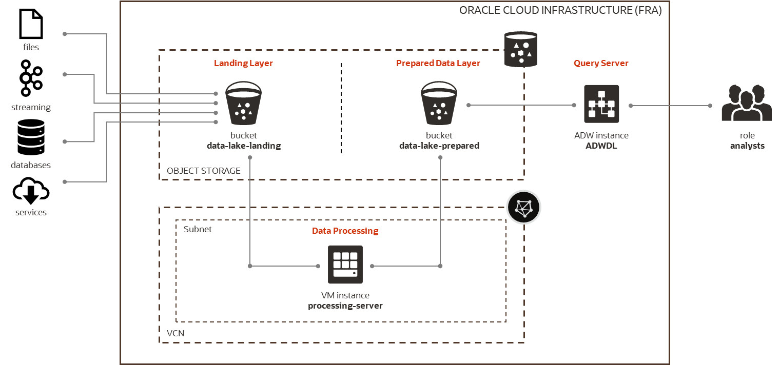
The architecture I used for the evaluation is simple. Data is collected from multiple internal and external sources and stored in the Data Lake. Data Lake consists of two layers. Landing Layer contains raw data from sources, while Prepared Data Layer contains data ready to be used by analytical users. Users are accessing Prepared Data to perform data discovery, analysis, data science, reporting, and to develop data-driven applications.

The Data Lake is implemented on Oracle Cloud Infrastructure (OCI). Data is managed in OCI Object Storage, with one bucket for Landing Layer and another bucket for Prepared Data Layer. Python modules running on OCI VM server are used for data processing and formatting. Autonomous Data Warehouse (ADW) and Python are used for data queries and analysis.

OCI VM server used for Python processing was running OL7, on VM.Standard2.1 shape (X7-based standard compute running 2.0 GHz Intel Xeon Platinum 8167M), with 1 OCPU (i.e. 1 core with 2 threads), 15 GB of memory and 1 Gbps network bandwidth.

Data

To test the file formats, I used an anonymized sample of HTTP log file, similar to one that could be generated by a service provider. The sample HTTP log is a text file, in standard CSV format. I tested 3 different sizes of the log file, to check if some formats behave differently based on file size.

Size	File	Format	Number of Records	Size (bytes)
Small	http_log_file_small.csv	CSV	39 824	8 297 419
Medium	http_log_file_medium.csv	CSV	199 120	43 658 389
Large	http_log_file_large.csv	CSV	1 075 248	238 551 316

The HTTP log file contains one row per each HTTP request. The information available in the log file is described in the following table.

#	Field	Description	Average Size (bytes)	Distinct Values %
1	start_time	Session start (Epoch time)	10,00	1,25%
2	end_time	Session end as (Epoch time)	10,00	0,19%
3	radius_calling_station_id	Calling station identifier	11,00	19,83%
4	ip_subscriber_ip_address	User IP address	13,88	19,85%
5	ip_server_ip_address	Server IP address	12,93	7,73%
6	http_host	Domain name	18,68	10,27%
7	http_content_type	Content type	15,32	0,65%
8	http_url	Request URL	78,16	71,12%
9	downlink_bytes	Downloaded bytes	4,84	30,21%
10	uplink_bytes	Uploaded bytes	4,83	6,26%
11	downlink_packets	Downloaded packets	2,83	1,03%
12	uplink_packets	Uploaded packets	2,82	0,10%
13	session_id	Session identifier	16,59	75,05%

Conversion

To test file formats, I converted the source files in Object Storage to multiple target files with different formats. The conversion process was fairly straightforward. A source file was downloaded from Object Storage using OCI API via Python SDK, converted into target format and schema, and uploaded back to Object Storage. The processing was done completely in memory, so that it could be implemented as serverless Oracle Function in the future.

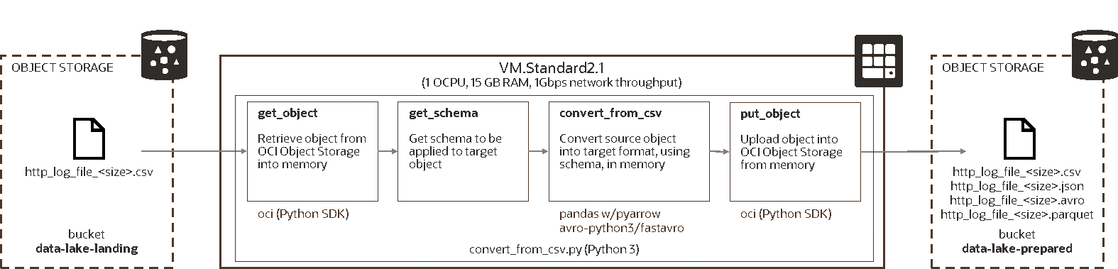
I used static schema and performed the conversion on adhoc basis with Python script. In a real-life Data Lake, schema should be managed by a schema registry (data catalog) and the conversion program would be invoked automatically, either triggered by arrival of source data or scheduled.

Scenarios

I tested conversion of HTTP log file into two text formats (CSV and JSON) and two binary formats (Avro and Parquet). For Parquet, I also tested snappy and gzip compression, in addition to no compression. For simplicity, I used Python pandas package for conversion where possible.

#	Description	Format	Compression	Method
1	Conversion to CSV (pandas)	CSV	None	pandas.to_csv()
2	Conversion to JSON (pandas)	JSON	None	pandas.to_json()
3	Conversion to Avro (avro-python3)	Avro	None	avro-python3.DataFileWriter()
4	Conversion to Avro (fastavro)	Avro	None	fastavro.writer()
5	Conversion to Parquet (pandas, uncompressed)	Parquet	None	pandas.to_parquet() w/pyarrow
6	Conversion to Parquet (pandas, snappy)	Parquet	snappy	pandas.to_parquet() w/pyarrow
7	Conversion to Parquet (pandas, gzip)	Parquet	Gzip	pandas.to_parquet() w/pyarrow

The selection of conversion scenarios requires some explanation.

• CSV, JSON, Avro, and Parquet are commonly used formats, no surprise there.

• I did not test ORC format as it is not well supported by Python and pandas.

• I did not test other formats supported by pandas as they are not supported by ADW.

• I did not test compression of CSV and JSON as pandas cannot do it in memory.

• I used two packages for Avro, as avro-python3 turned out to be very slow.

File Size

The first test answers how efficient are different formats and compression methods. Or, in other words, how much space a file format requires. Of course, the smaller is better – the less space is needed, the faster you access or upload data over the network, the less you pay for storage, the easier it is to manage data.

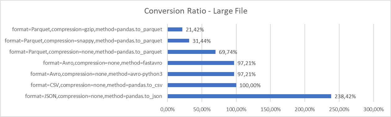
The following graph shows conversion ratios for large file. 100% is CSV format (i.e. source). Ratio smaller than 100% means more efficient storage than CSV, higher than 100% means less efficient storage. Note the ratios for medium and small files are similar and hence I do not show them.

• Not surprisingly, Parquet, as a columnar store, is the most storage efficient format. With gzip compression, we can get to 21% of the original size. Snappy compression is slightly worse but still good, with 31% of the original size.

• Avro has similar storage efficiency as CSV format, with 97% of the original size. I suppose Avro would be more efficient if we use more non-string data types such as int and long, but this remains to be tested in the future.

• JSON is the least efficient format. With JSON, the file size explodes to 2.5 times the original CSV file. The size could be decreased by using more terse names of JSON fields, but the JSON file would be still significantly larger than CSV or Avro files.

Throughput

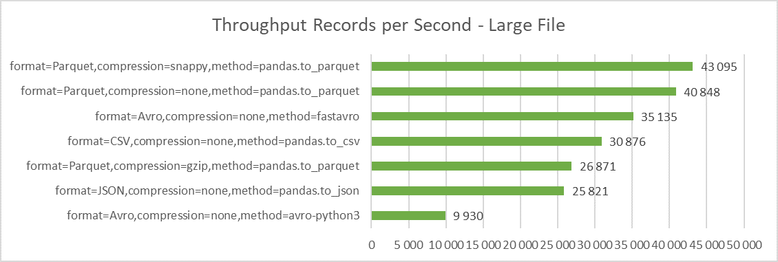
The second test looks at how many records we are able to convert in a second. Although this measure is very data specific, I believe it is much more informative for most data processing scenarios than bytes per second, since we can directly relate number of records to number of business events. Ability to process and publish data quickly is essential in current data driven architectures.

As explained in the Conversion section, I look at the whole process, including not just the conversion itself, but also time it takes to get the source from Object Storage and write the converted file back to Object Storage. Also please note the figures are for single file and single threaded process.

• The best throughput delivers pandas/pyarrow with Parquet format and snappy compression, with 43k lines per second (25 seconds for large file, 4.7 seconds for medium file) respectively. This clearly shows that while gzip compress files more efficiently, snappy performs the compression significantly faster.

• The Avro format prepared with fastavro package also delivers respectable performance, with 35k lines per second (30 seconds for large file). This is in sharp contrast with avro-python3 package, which has by far the lowest performance and is therefore almost useless.

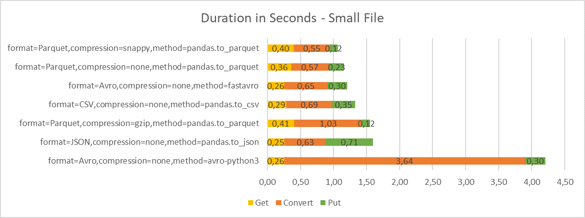
• For small files, the throughput is somewhat worse, with 37k lines per second for Parquet/snappy. This is caused by higher impact of reading and writing to Object Storage compared to conversion itself, as discussed in the next section.

Duration

The next test looks at the duration of the conversion process and break-down to individual phases. I have included graphs for all three file sizes to illustrate the impact on donwloading and uploading data from Object Storage on the overall duration. Note that downloading the source file from Object Storage should have on average the same duration regardless of scenario.

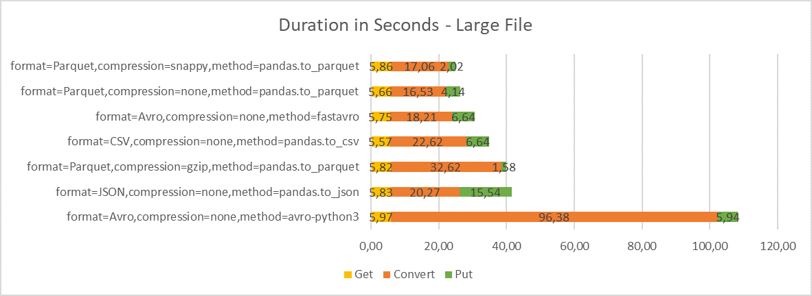
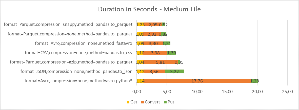
• Although the conversion step takes most time (between 60-80% for larger files, depending on the method), reading and writing data from and to Object Storage is also significant.

• When reading data from Object Storage, I observed consistent throughput of about 39-40 MBps for larger files. For writing data, the throughput is more volatile – 32-39 MBps. The throughput is constrained by Object Storage performance for single request. We could get significantly better throughput for parallel requests or multi-part uploads.

• Note that in our case both processing server and Object Storage are in the same OCI region. With server outside the OCI region, the get/put operations would take much longer.

• For Parquet format with gzip compression, you can clearly see how much the snappy compression is faster than gzip compression. This is somewhat alleviated by faster upload but not by much.

• For JSON, you can see that while the conversion to JSON with pandas is pretty fast, the upload to Object Storage caused by large file size takes significant part of the overall time.

Memory

The last file conversion measure I evaluated is the amount of memory needed by the conversion process. This measure is important for environments with limited resources; such as Docker containers running on Oracle Functions serverless platform. These environments have reduced amount of available memory; when the function exceeds the shape memory, its execution is stopped. For example, Oracle Functions support maximum of 1024 MB.

Note that the memory consumption was measured by tracking the maximum resident set size (RSS) as provided by resource.getrusage() call in Python at the end of the program.

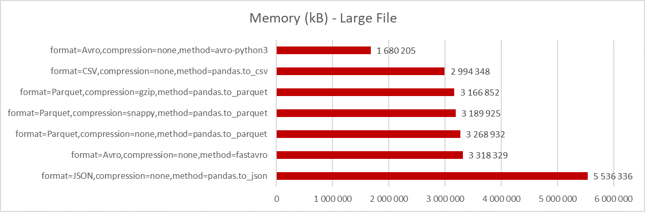
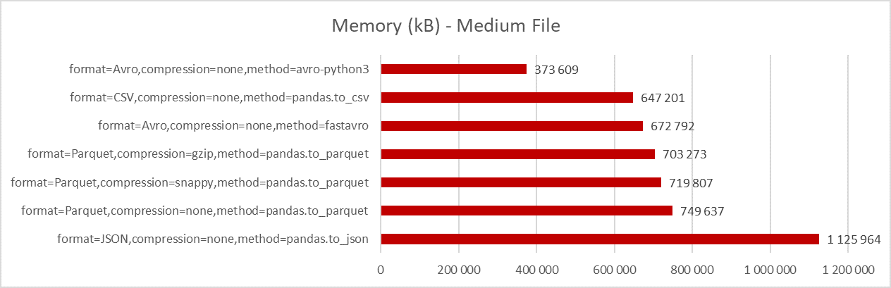
• You can see that avro-python3 package requires the least memory. This is caused by the fact that this package needs only 2 copies of data in memory – source (CSV) and target (Avro). With avro-python3 you can directly stream to target Avro object.

• On the other hand, pandas and fastavro need 3 copies of data in the memory – the source object, dataframe (or array in case of fastavro), and the target object. To reduce the memory, we would need to find a way to directly convert source to target, bypassing the dataframe.

• The memory required for conversion of large files clearly exceeds the memory limit available for Oracle Functions, even in case of avro-python3 package. Note I have not tested other conversion libraries and languages which might have more efficient memory handling.

Summary

This concludes the part focusing on storage efficiency and conversion performance. The key findings are as follows.

• Parquet with snappy compression provides the best compromise between the space requirements and processing speed. This would be my default selection for prepared data.

• Parquet with gzip compression delivers the most efficient compression. If space savings are the priority, this would be the preferred choice.

• I do not see much use for Avro and CSV, at least for our use case. They require significantly more space than Parquet and the conversion speed is also somewhat worse than Parquet.

• JSON should not be used for larger files at all, because of space explosion. You should consider it only for small files that must be human readable.

• Take care when doing the conversion on platform with restricted memory, such as Oracle Functions, as larger files will not fit into available memory shapes.

• Measurements in this post depend on the sample data, processing server configuration and also on the Python conversion code. Your mileage will vary!

The second part of this post will look at how fast we can access and analyze prepared data in Object Storage, using Autonomous Data Warehouse and Python/pandas. Stay tuned!